1. Introduction

 

All over the world, environmental pollution is one of the most dangerous issues (Amasha and Aly, 2019; Elnour et al., 2018; Singh and Kapoor, 2019). In a monitoring program, a mathematical simulation of gas emission is quite essential when the gas modeled is toxic. Toxicity due to gas must not be common and when happened is surely an accident, where a quick diagnostic must be necessary for avoiding fatal losses (Rigas and Sklavounos 2007). When in an emission monitoring program, the goal is to keep these at minimum levels but due to a human error or just an accident (old machinery, rusted pipes, extreme pressure, toxic substances spills, etc.), the pollutant concentration in air can be out of boundaries. These accident cases could occur in the mines, chemicals, or other transformation industries (Maria and Markiewicz, 2012). Besides, the monitoring programs in some legislations (as the Mexican), for the environmental impact studies, a risk analysis is required and in the popular methods suggested like ALOHA® (Fedra, 1998), the simulation is Gaussian and the number of substances modeled is limited. Because of that, this paper proposal is to study instant emissions of extreme concentration pollutants. This is necessary to define the impact area and the contamination levels that may occur in an industry or any given área because modeling helps to build legislation and measurements to protect the environment. On the other hand, pollutant sources may be human-created or naturals; in this second case, it is important to generate evacuation plans according to the modeling to save most lives as possible and to avoid panic or unnecessary emigrations that just cost money and time in better scenarios.

The model we worked with is based on the mass transfer and in this research, the mathematical expression is (Bird et al. 2002):

 

 

Where cr,t  is the pollutant concentration that depends on the location and the time, D  is the diffusivity, and v  is the velocity of the wind. It must be clear that this model does not contemplate chemical reactions nor other kinds of interaction with other gasses. The pollutant dispersion in the atmosphere is dominated by two mechanisms (Wark, 1981), the air flux and turbulences; these scatter the pollutants in all directions.

The pollutant transfer is, in general, a complex problem; it relays on many factors such as gas and air temperature, moisture, etc. There is a methodology (Pasquill method) to analyze the air dispersion classifying it using its thermodynamics’ conditions, including temperature. If the airspeed is under 2 m/s, it is considered to be low. The main problem with this is that at low-speed Pasquill method supposes that pollutants remain static and this is very interesting to study this case (Sharan et al. 1996; table 1).

 

Table 1. Atmosphere stability classes in accordance with Pasquill (Sharan, et al. 1996).

Wind velocity on the height	Daytime, incoming solar radiation			Night, cloudiness
of 10m (m/s)	Strong	Moderate	Weak	Clouded	Cloudless
< 2	A	A – B	B	E	F
2 - 3	A – B	B	C	E	F
3 - 5	B	B – C	C	D	E
5 - 6	C	C – D	D	D	D
> 6	C	D	D	D	D

 

The main objective of this paper is to calculate the dispersion of pollutants using two methods via Fourier transform for some cases: instantaneous point source, continuous point source, several instantaneous points sources, a finite source of time, and finally, a linear source.

 

2. Theory

One of the techniques to analyze the dynamic behavior of dynamic systems is the Fourier transform (Weber and Arfken, 2003). The Fourier transform is a linear transformation that allows studying a system either in the time domain or in the frequency; said transformation is defined as:

 

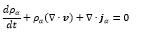
This allows studying a system that is complicated in time but not in frequency; a reason why transformations like Fourier's or Laplace's make the description easier in many cases (Weber and Arfken, 2003). On the other hand, one of the fundamental principles of nature is that the mass is conserved and writing this in equations gives the equation of continuity (Welty et al. 2014):

 

If we define  ji=ρi(vi-v)  then:

 

 

In the experiments, it is easier to talk about the concentration of the substance in the binding of the densities,

 

or

 

In thermodynamics, the concept of chemical potential μ is introduced and in the context of transport we can establish that a system that is not in chemical equilibrium (Levich et al. 1978), there will be a mass flow so we will take that:

 

j=-γ∇μ

 

Taking an isothermal process in the event that μ=μ(p,cα) , then

 

 

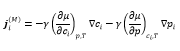
It has been proposed then that diffusion is due to two causes, a concentration and pressure gradient, which agrees with the experiment. However, it is possible to induce transport via temperature gradient or electromagnetic fields (Welty et al. 2014). We define the molecular diffusion coefficient and the pressure coefficient as:

 

 

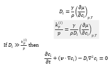
The last expression is called Fick's Second Law (Levich et al. 1978).

 

3. Results

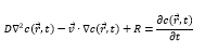
Pollutants’ transfer in the air can be described by the next equation:

 

(1)

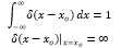
In the anterior expressions may be referred to as a source or a sink, are the speed of the air and is the concentration of the pollutant. The sources may be punctual, lineal, or by area whose can be simulated like a Dirac delta. In general, Dirac delta generalized functions are used to simulate sources due to incidents (Weber and Arfken, 2003). The Dirac Delta Function is defined as:

 

(2)

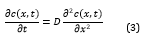
Rewritten the equation (1) assuming no chemical reaction and the velocity of the air is too low, so we are going to study instantaneous emission in one dimension and after that in several dimensions with and without wind, so several cases we are going to study.

 

1. Instantaneous emission with no wind

 

(3)

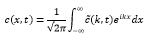
To solve the last equation will be solved by using the Fourier transform:

 

cx,t=1√2π-∞∞ck,teikxdx

(4)

 Substituting equation (3) into (4) we obtain

∂C(x,t)∂t=-k2DC(k,t)

(5)

where the solution is

 

Ck,t=A(k)e-k2Dt

(6)

The source of contamination will be given as an initial condition of the system

 

Cx,0=fx=12π-∞∞Ck,0eikxdk

(7)

Being the inverse Fourier transform

 

Ck,0=12π-∞∞f(x)e-ikx

(8)

From equation (7) is obtained

 

Ck,0=Ak

(9)

Then

 

Ak=12π-∞∞fxe-ikx dx

(10)

 

 

 

With the last result, the solution of the equation is

 

Ck,t=12π-∞∞f(x)e-ikxe-kDtdx

(11)

Then, equation (5) in (9) is generated

 

Cx,t=12π-∞∞f(x)dx'-∞∞e-k2Dteikx'eikx

(12)

 

Since

 

-∞∞e-k2Dt+ik(x-x´)dk=√πe-(x-x')24DtDt

(13)

The above is demonstrated later; equation (35-43) So,

 

Cx,t=14πDt-∞∞Cx',0e-x-x'24Dtdx'

(14)

 

To model an instantaneous point source, for example an explosion, the Dirac Delta function is used:

 

Cx',0=mδ(x'-x)

(15)

Finally, the dispersion of the contaminant will be given by the equation

 

Cx,t=14πDtme-(x-x0')24Dt

(16)

This solution has been used in the environmental area to analyze the behavior of pollutants at the low velocity of the air. Observation: the units of C are mass/length, so we should incorporate the transversal área, this means that

 

Cx,t=1A4πDtme-(x-x0')24Dt

 

2. Instantaneous emission with wind

 

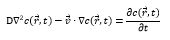
To consider the effects of wind speed, the differential equation that describes the pollutant under these conditions we have

 

∂c(x,t)∂t=D∂2c(x,t)∂x2-u∂c(x,t)∂t

(17)

 

The easiest is to make a change of variable

 

ε=x-ut

(18)

 

Then,

 

∂c∂x=∂c∂ε∂ε∂x+∂c∂t∂t∂t=∂c∂ε

(19)

 

Finally,

 

∂2c∂x2=∂2c∂ε2

(20)

When considering the derivative with respect to time we have

 

∂c∂t=∂c∂ε∂ε∂t+∂c∂t∂t∂t=-u∂c∂ε+∂c∂t

(21)

 

Then,

 

∂c(x,t)∂t=D∂2c(x,t)∂ε2

(22)

 

The solution of equation 22 is

 

cx,t=m4πDte-ε24Dt=m4πDte-(x-ut)24Dt	(23)
Instanateous point source several dimensión with wind

 

In two dimension is a similar way

 

D∂2c(x,y,t)∂x2+∂2c(x,y,t)∂y2=∂c(x,y,t)∂t	(24)

Applying the Fourier transform we obtain

 

cx,y,t=12π-∞∞dkxdkyc(kx,ky,t)eikxxeikyy

(25)

 

It is worth mentioning that we will change the notation c=c(kx,ky,t) , and when substituting in the differential equation we obtain

 

D-kx2-ky2c=∂c∂t

(26)

The general solution of the first-order linear differential equation is

 

c=A(kx,ky)e-Dkx2+ky2t

(27)

The source of contamination would be given as an initial condition

 

cx,y,0=fx,y=12π-∞∞dkxdkyc(kx,ky,0)eikxxeikyy

(28)

 

The inverse transform

 

c=12π-∞∞dxdyf(x,y)e-ikxxe-ikyy

(29)

 

Then, we define

 

 

	Akx,ky=12π-∞∞dxdyf(x,y)e-ikxxe-ikyy	(30)
	The solution of the equation (24) is
	c(kx,ky,t)=12π-∞∞dxdyf(x,y)e-ikxxe-kx2Dte-ikyye-ky2Dt	(31)
	or
c(x,y,t)=12π2-∞∞dx'dy'f(x',y')-∞∞dkxdkyeikxx-ikxx'e-kx2Dteikyy-ikyy'e-ky2Dt		(33)

 

Furthermore,

 

-∞∞e-k2Dt+ik(x-x´)dk=√πe-(x-x')24DtDt

(34)

 

To demonstrate the above we must complete the perfect square binomial

 

 

-k2Dt+ikx-x´=-Dt[k2-ikDtx-x'+14D2t2x-x'2-14D2t2x-x'2]

(35)

 

Then,

 

-k2Dt+ikx-x´=-14Dtx-x'2[k-i(x-x')2Dt]2

(36)

 

Substituting this in the integral

 

-∞∞e-14Dtx-x'2[k-i(x-x')2Dt]2dk=e-14Dtx-x'2-∞∞e-Dt[k-i(x-x')2Dt]2dk=√πe-(x-x')24DtDt

(37)

 

The integral of has the form

 

 

-∞∞e-az2dz=πa

(38)

We define

 

I=-∞∞e-ax2dx=-∞∞e-ay2dy

(39)

 

 

Then,

I2=-∞∞e-a(x2+y2)dxdy

(40)

Making the change to polar coordinates we obtain

 

-∞∞e-a(x2+y2)dxdy=0∞02πe-ar2rdrdθ=2π0∞e-ar2rdr

(41)

 

 

0∞e-ar2rdr=-12ae-ar20∞=12a

(42)

 

Finally,

I=πa

(43)

We obtain that

 

c(x,y,t)=14πDt-∞∞dx'dy'cx',y',0e-(x-x')24Dte-(y-y')24Dt

(44)

 

Taking as a Dirac Delta type source,

 

cx',y',0=mδ(x'-x0)δ(y'-y0)

(46)

 

This leads to

 

c(x,y,t)=m4πDte-(x-x0)24Dte-(y-y0)24Dt	(47)
In general,
c(x,y,z,t)=m4πDt3/2e-(x-ut)24Dte-(y-vt)24Dte-(z-H)24Dt	(48)

 

If we define

4Dt=2σ2

(49)

 

The general solution is given the σ  parameter

 

σ=2Dt	(50)

The equation (48) is now of the form

 

c(x,y,z,t)=m2π3/2σxσyσze-(x-ut)22σx2e-(y-vt)22σy2e-(z-H)22σz2	(51)
Several instantataneous point sources

In the case of two sources, we use the Dirac Delta for two different sites

 

cx',y',0=m0δx'-x0δy'-y0+m1δx'-x1δy'-y1

(52)

Then,

 

cx,y,z,t=m02π32σx0σy0σz0e-x-ut22σx02e-y-vt22σy02e-z-H022σz02 +m12π3/2σx1σy1σz1e-(x-x1-ut)22σx12e-(y-y1-vt)22σy12e-(z-H1)22σz12

(53)

If we have several sources,

 

cx,y,z,t=i=1nmi2π3/2σxiσyiσzie-(x-xi-ut)22σxi2e-(y-yi-vt)22σyi2e-(z-Hi)22σzi2

(54)

 

5. Point source emission at a certain time

Palazzi and colleagues (Palazzi et al. 1982) developed a theory about difusión of pollution in a short time. In this section, step by step we developed the model.

 

c(x,y,z)=0tq2π32σxσyσze-x-ut'22σx2e-y22σy2e-z-H22σz2dt'

(66)

 

And x'=ut'  then,

 

c(x,y,z)=0∞q2π32σxσyσze-x-ut'22σx2e-y22σy2e-z-H22σz2dt'

(67)

 

We define α=x-ut'2σx

 

cx,y,z=-2q2π32σyσzue-y22σy2e-z-H22σz2x2σx-∞e-α2dα

(68)

 

Or

 

c(x,y,z)=q4πσyσzue-y22σy2e-z-H22σz22σxπ2erfc(-x2σx)

(70)

 

It is very important to note that when t→∞ , then x2σx→∞  so

 

c(x,y,z)=q2πσyσzue-y22σy2e-z-H22σz2

(71)

 

When we have inversion problem, then

 

c(x,y,z)=q2πσyσzue-y22σy2(e-z-H22σz2+e-z+H22σz2)

(72)

 

If z=0 , this means on the ground

 

c(x,y,z)=qπσyσzue-y22σy2e-H22σz2

(73)

 

On the other hand, by tanking α=x-ut'2σx

 

cx,y,z=-2q2π32σyσzue-y22σy2e-z-H22σz2x2σxx-uT2σxe-α2dα

(74)

 

Then,

 

cx,y,z=-2q2π32σyσzue-y22σy2e-z-H22σz2x2σxx-uT2σxe-α2dα

(75)

 

Let see

 

x2σxx-uT2σxe-α2dα=x2σx0e-α2dα+0x-uT2σxe-α2dα=-0x2σxe-α2dα+0x-uT2σxe-α2dα

(76)

 

Finally,

 

cx,y,z=-2q2π32σyσzue-y22σy2e-z-H22σz2(-0x2σxe-α2dα+0x-uT2σxe-α2dα)

(77)

By using the error function described in Weber and Arfken (2003),

 

erfz=2π0ze-x2dx	(78)
Then,
cx,y,z=q4πσyσzue-y22σy2e-z-H22σz2 [erfx2σx-erf⁡(x-uT2σx)]	(80)

The above is valid for when the sources are finite at the time where T is the emission time. For times greater than or equal to T we have

 

cx,y,z=q4πσyσzue-y22σy2e-z-H22σz2 [erfx-u(t-T)2σx-erf⁡(x-uT2σx)]

(81)

 

Equations 80 and 81 are the same results that Palazzi et al (1982) obtained.

 

6. Linear pollution source

 

To study linear sources we will use the superposition principle with a constant concentration along the line. So, we have

 

c(x,y,z,t)=m02π3/2σxσyσze-(x-ut)22σx2e-(y-vt)22σy2e-(z-H)22σz2

(82)

 

Integrating with respect y  in the interval [-a,a]  and assuming that v=0  we have

 

c(x,y,z,t)=m02π3/2σxσyσze-(x-ut)22σx2e-(z-H)22σz2-aae-12yσy2dy

(83)

 

To solve this integral, special functions are used that are called the error function or numerically (Weber and Arfken, 2003). On the other hand, are parameters that represent the dispersion coefficients and they depend on environmental factors used in Briggs’s equations as shown in table 2 (Arystanbekova, 2004).

 

Table 2. Briggs’ formulae for defining plume semi-width.

Atmosphere stability class in accordance with Pasquill	σx,σy (m)	σz (m)
Open country
A	0.22X (1 + 0.0001 X)-1/2	0.2 X
B	0.16X (1 + 0.0001 X)-1/2	0.12 X
C	0.11X (1 + 0.0001 X)-1/2	0.08X (1 + 0.0002 X)-1/2
D	0.08X (1 + 0.0001 X)-1/2	0.06X (1 + 0.0015 X)-1/2
E	0.06X (1 + 0.0001 X)-1/2	0.03X (1 + 0.0003 X)-1
F	0.04X (1 + 0.0001 X)-1/2	0.016X (1 + 0.0003 X)-1
City
A-B	0.32X (1 + 0.0004 X)-1/2	0.24X (1 + 0.001 X)
C	0.22X (1 + 0.0004 X)-1/2	0.2 X
D	0.16X (1 + 0.0004 X)-1/2	0.14X (1 + 0.0003 X)-1/2
E-F	0.11X (1 + 0.0004 X)-1/2	0.08X (1 + 0.0015 X)-1/2
Here X  is the distance from the stack along with the plume ax.

 

4. Conclusion

The transport of pollutants is done by studying differential equations and semi-empirical proposals with which packages such as ALOHA are made. In this work we described via the conservation of mass equation and, Fick's law, which is an empirical proposal, the transport of a pollutant in the air. Also, the goodness of working with the Fourier transform was shown. As a proposal of the work, it is to include this type of development in the courses of simulation of environmental systems or the course of air quality so that the student understands the support of the programs like ALOHA and, to see an application of the courses of differential equations and Physics.

REFERENCES

1. Amasha, R. H. & Aly M. M. (2019). Removal of Dangerous Heavy Metal and Some Human Pathogens by Dried Green Algae Collected from Jeddah Coast. Pharmacophore, 10(3), 5-13.
2. Arystanbekova, N. K. (2004). Application of Gaussian plume models for air pollution simulation at instantaneous emissions. Mathematics and Computers in Simulation, 67(4-5), 451-458.
3. Bird, R. B., Steward, W. E., & Lightfoot, E. N. (1987). Transport Phenomena, 2nd Edition, John Wiley & Sons. 2002.
4. Elnour, A. A., Abdelfattah, M. M., Negm, S. & Kassim, T. (2018). Microbiological Surveillance of Air Quality: A comparative Study Using Active and Passive Methods in Operative Theater. International Journal of Pharmaceutical and Phytopharmacological Research, 8(1), 33-38.
5. Fedra K. (1998). Integrated risk assessment and management: overview and state of the art. Journal of Hazardous Materials, (61), 1–3.
6. Levich, V. G., Vdovin, I. A., & Miamlin, V. A. (1978). Curso de Física Teórica, Volumen 4: Estadística Cuántica y Cinética Física. Ed. Reverté SA, Buenos Aires, Argentina.
7. Maria T., & Markiewicz. (2012). A review of mathematical models for the atmospheric dispersion of heavy gases Part I. A Classification of models. Ecological Chemistry and Engineering S. 19 (3): 297-314.
8. Palazzi, E., De Faveri, M., Fumarola, G., & Ferraiolo, G. (1982). Diffusion from a steady source of short duration. Atmospheric Environment, 16(12), 2785-2790.
9. Rigas F, & Sklavounos S. (2007). Computer simulation in consequence analysis and loss prevention. In: New research on hazardous materials. Warrey PB, editors. Nova Science Publishing Inc. 161-20
10. Sharan M., Yadar A. K., Singh M. P., Agarwal P. & Nigam S. (1996). A mathematical model for the dispersion for air pollutants in low wind conditions. Atmospheric Environment 30 (8), 1209-1220.
11. Singh, J. & Kapoor, R. K. (2019). Immobilization and Reusability Efficiency of Laccase Onto Different Matrices Using Different Approaches. International Journal of Pharmaceutical and Phytopharmacological Research, 9(1), 58-65.
12. Wark, (1981). Kenneth Wark and Cecil Warner, “Air Pollution: Its Origin and Control,” HarperCollins, New York, NY, 1981.
13. Weber, H. J., & Arfken, G. B. (2003). Essential mathematical methods for physicists, ISE. Elsevier.
14. Welty, J., Rorrer, G. L., & Foster, D. G. (2014). Fundamentals of momentum, heat, and mass transfer. John Wiley & Sons.